

实践一
任务1:dominates(a,b)数实现
任务2:Archive管理(加入、删除、拥挤选点)
任务 3:Leader Selection(任选一个方法)
任务4:绘制不同选代的前沿图
代码
import numpy as np
import matplotlib.pyplot as plt
import random
# --- 基础设置 ---
class Particle:
def __init__(self, dim):
self.position = np.random.rand(dim) # ZDT1 范围 [0, 1]
self.velocity = np.zeros(dim)
self.best_position = self.position.copy()
self.fitness = None
self.best_fitness = None
# ZDT1 测试函数 (2个目标)
def zdt1(x):
f1 = x[0]
g = 1 + 9 * np.sum(x[1:]) / (len(x) - 1)
h = 1 - np.sqrt(f1 / g)
f2 = g * h
return np.array([f1, f2])
# ==========================================
# 任务 1: dominates(a, b) 函数实现
# ==========================================
def dominates(fitness_a, fitness_b):
"""
判断解 a 是否支配解 b
条件: a 在所有目标上 <= b,且至少有一个目标 < b (假设是最小化问题)
"""
all_better_or_equal = np.all(fitness_a <= fitness_b)
one_strictly_better = np.any(fitness_a < fitness_b)
return all_better_or_equal and one_strictly_better
# ==========================================
# 任务 2: Archive 管理 (加入、删除、拥挤选点)
# ==========================================
def calculate_crowding_distance(archive_fitness):
"""简化的拥挤度计算,用于维护 Archive 多样性"""
l = len(archive_fitness)
if l == 0: return []
distances = np.zeros(l)
# 按每个目标排序并计算距离
num_objs = len(archive_fitness[0])
for m in range(num_objs):
sorted_indices = np.argsort(archive_fitness[:, m])
# 边界点距离设为无穷大
distances[sorted_indices[0]] = np.inf
distances[sorted_indices[-1]] = np.inf
f_min = archive_fitness[sorted_indices[0], m]
f_max = archive_fitness[sorted_indices[-1], m]
if f_max == f_min: continue
# 中间点计算
for i in range(1, l - 1):
distances[sorted_indices[i]] += (archive_fitness[sorted_indices[i+1], m] - archive_fitness[sorted_indices[i-1], m]) / (f_max - f_min)
return distances
def update_archive(archive, particle, capacity=100):
"""
Archive 管理核心逻辑:
1. 如果新粒子被 Archive 中任意成员支配 -> 忽略
2. 如果新粒子支配 Archive 中成员 -> 删除被支配成员,加入新粒子
3. 如果互不支配 -> 加入新粒子
4. 如果 Archive 满了 -> 使用拥挤度删除最拥挤的
"""
p_fit = particle.fitness
p_pos = particle.position.copy()
# 检查是否被支配
for member in archive:
if dominates(member['fitness'], p_fit):
return archive # 被支配,不加入
# 删除被新粒子支配的成员
# 使用列表推导式保留未被 p 支配的
new_archive = [m for m in archive if not dominates(p_fit, m['fitness'])]
# 加入新粒子
new_archive.append({'position': p_pos, 'fitness': p_fit})
# 拥挤度维护 (如果超过容量)
if len(new_archive) > capacity:
# 提取所有 fitness 用于计算
fits = np.array([m['fitness'] for m in new_archive])
dists = calculate_crowding_distance(fits)
# 删除拥挤度最小的 (最拥挤的),但在排序中要小心处理无穷大
# 既然我们要保留距离大的,那就删除距离最小的
min_idx = np.argmin(dists)
new_archive.pop(min_idx)
return new_archive
# ==========================================
# 任务 3: Leader Selection (任选一个方法)
# ==========================================
def select_leader(archive):
"""
从 Archive 中选择全局最优 (gbest)。
这里使用【随机选择】。
"""
if not archive:
return None
# 基于拥挤度选择(越稀疏被选概率越大),这里用简单随机
selected = random.choice(archive)
return selected['position']
# ==========================================
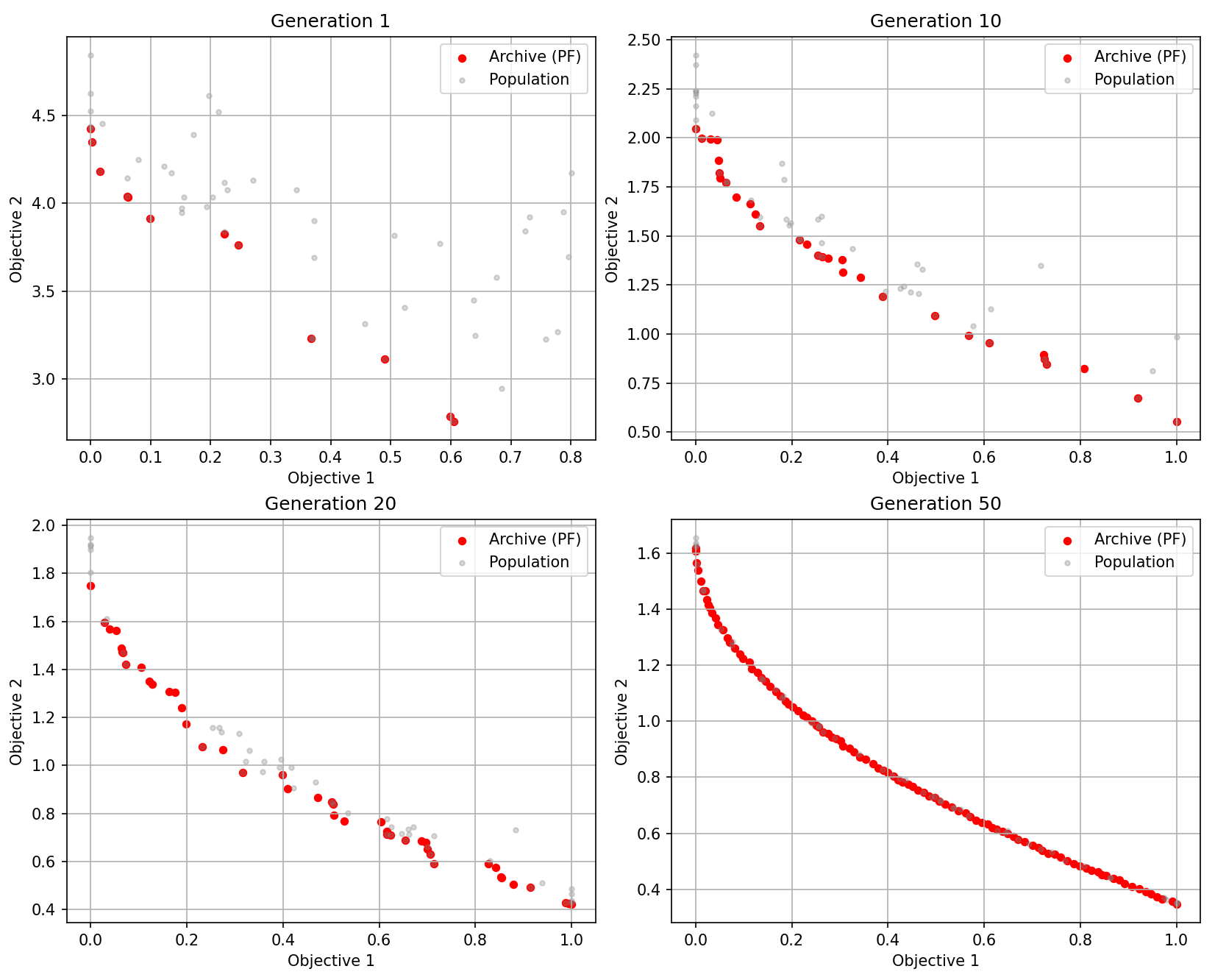
# 任务 4: 绘制不同迭代的前沿图 & 主循环
# ==========================================
def run_mopso():
# 参数设置
dim = 30
pop_size = 50
max_iter = 50 # 对应题目要求的 50 代
archive_capacity = 100
w, c1, c2 = 0.5, 1.5, 1.5 # 惯性权重和学习因子
# 初始化种群
population = [Particle(dim) for _ in range(pop_size)]
archive = []
# 初始化评估
for p in population:
p.fitness = zdt1(p.position)
p.best_fitness = p.fitness
archive = update_archive(archive, p, archive_capacity)
# 绘图准备
plot_iters = [1, 10, 20, 50]
fig, axs = plt.subplots(2, 2, figsize=(12, 10))
axs = axs.flatten()
plot_idx = 0
print("开始迭代...")
for iteration in range(1, max_iter + 1):
for p in population:
# Task 3: 选择 Leader
gbest_pos = select_leader(archive)
if gbest_pos is not None:
# 更新速度和位置
r1, r2 = np.random.rand(), np.random.rand()
p.velocity = (w * p.velocity +
c1 * r1 * (p.best_position - p.position) +
c2 * r2 * (gbest_pos - p.position))
p.position = p.position + p.velocity
# 越界处理 (简单的截断)
p.position = np.clip(p.position, 0, 1)
# 评估
current_fitness = zdt1(p.position)
p.fitness = current_fitness
# 更新个体最优 pbest
if dominates(current_fitness, p.best_fitness):
p.best_position = p.position.copy()
p.best_fitness = current_fitness
elif not dominates(p.best_fitness, current_fitness):
# 互不支配时,随机选一个或者保留旧的,这里简单处理:保留旧的
if np.random.rand() < 0.5:
p.best_position = p.position.copy()
p.best_fitness = current_fitness
# Task 2: 更新 Archive
archive = update_archive(archive, p, archive_capacity)
# 打印进度
print(f"Generation {iteration}, Archive Size: {len(archive)}")
# Task 4: 绘图
if iteration in plot_iters:
ax = axs[plot_idx]
# 提取 Archive 中的 fitness 进行绘制
archive_fits = np.array([m['fitness'] for m in archive])
if len(archive_fits) > 0:
ax.scatter(archive_fits[:, 0], archive_fits[:, 1], c='red', s=20, label='Archive (PF)')
# 也可以画出当前种群作为背景(灰色)
pop_fits = np.array([p.fitness for p in population])
ax.scatter(pop_fits[:, 0], pop_fits[:, 1], c='gray', alpha=0.3, s=10, label='Population')
ax.set_title(f"Generation {iteration}")
ax.set_xlabel("Objective 1")
ax.set_ylabel("Objective 2")
ax.legend()
ax.grid(True)
plot_idx += 1
plt.tight_layout()
plt.show()
# 运行
if __name__ == "__main__":
run_mopso()输出
开始迭代...
Generation 1, Archive Size: 12
Generation 2, Archive Size: 5
Generation 3, Archive Size: 7
Generation 4, Archive Size: 21
Generation 5, Archive Size: 19
Generation 6, Archive Size: 18
Generation 7, Archive Size: 22
Generation 8, Archive Size: 21
Generation 9, Archive Size: 26
Generation 10, Archive Size: 30
Generation 11, Archive Size: 33
Generation 12, Archive Size: 32
Generation 13, Archive Size: 30
Generation 14, Archive Size: 29
Generation 15, Archive Size: 36
Generation 16, Archive Size: 37
Generation 17, Archive Size: 42
Generation 18, Archive Size: 54
Generation 19, Archive Size: 52
Generation 20, Archive Size: 44
Generation 21, Archive Size: 43
Generation 22, Archive Size: 43
Generation 23, Archive Size: 40
Generation 24, Archive Size: 43
Generation 25, Archive Size: 44
Generation 26, Archive Size: 57
Generation 27, Archive Size: 63
Generation 28, Archive Size: 64
Generation 29, Archive Size: 66
Generation 30, Archive Size: 71
Generation 31, Archive Size: 83
Generation 32, Archive Size: 93
Generation 33, Archive Size: 100
Generation 34, Archive Size: 100
Generation 35, Archive Size: 100
Generation 36, Archive Size: 100
Generation 37, Archive Size: 100
Generation 38, Archive Size: 100
Generation 39, Archive Size: 100
Generation 40, Archive Size: 100
Generation 41, Archive Size: 100
Generation 42, Archive Size: 100
Generation 43, Archive Size: 100
Generation 44, Archive Size: 100
Generation 45, Archive Size: 100
Generation 46, Archive Size: 100
Generation 47, Archive Size: 100
Generation 48, Archive Size: 100
Generation 49, Archive Size: 100
Generation 50, Archive Size: 100
可视化
实践二
作务1:dominates(a,b)所数
作务2:实现 DE mutation
任务3:更新档案库(增加/除/挤距离)
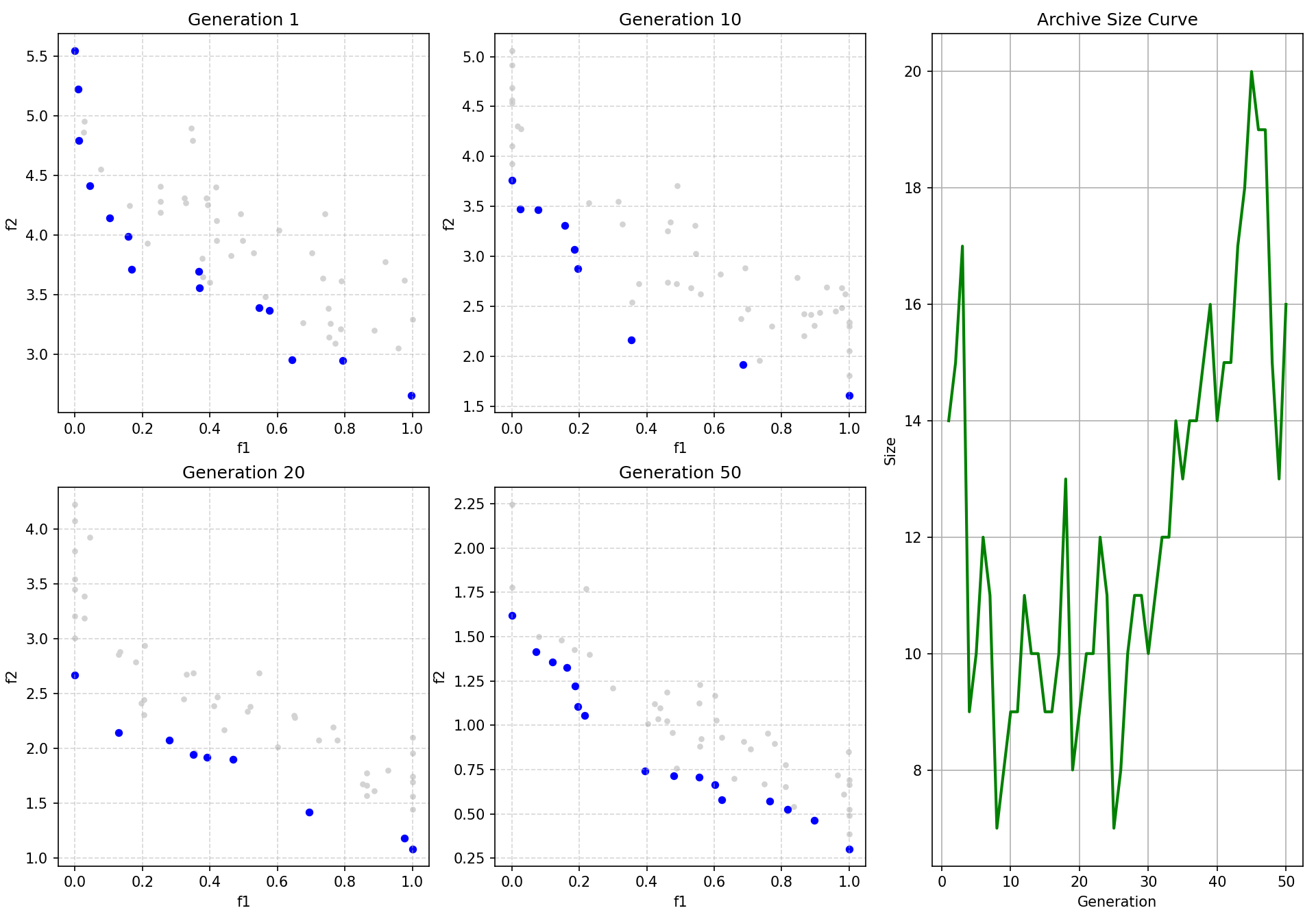
作务4:绘制Pareto 前(每10代一次)
要求提交:
-
10、20、50 代前沿图
-
档案库大小曲线
-
100 字短文:MODE VS NSGA-II:谁更稳定? 谁更快?
代码
import numpy as np
import matplotlib.pyplot as plt
import random

# --- 基础设置: ZDT1 测试函数 ---
def zdt1(x):
    dim = len(x)
    f1 = x[0]
    g = 1 + 9 * np.sum(x[1:]) / (dim - 1)
    h = 1 - np.sqrt(f1 / g)
    f2 = g * h
    return np.array([f1, f2])

# ==========================================
# 任务 1: dominates(a, b) 函数实现
# ==========================================
def dominates(fit_a, fit_b):
    """如果 a 支配 b 返回 True"""
    return np.all(fit_a <= fit_b) and np.any(fit_a < fit_b)

# ==========================================
# 任务 3: Archive 管理 (增加/删除/拥挤距离)
# ==========================================
def calculate_crowding_distance(archive_fits):
    l = len(archive_fits)
    if l == 0: return []
    distances = np.zeros(l)
    num_objs = len(archive_fits[0])

    for m in range(num_objs):
        sorted_indices = np.argsort(archive_fits[:, m])
        distances[sorted_indices[0]] = np.inf
        distances[sorted_indices[-1]] = np.inf

        f_min = archive_fits[sorted_indices[0], m]
        f_max = archive_fits[sorted_indices[-1], m]
        if f_max == f_min: continue

        for i in range(1, l - 1):
            distances[sorted_indices[i]] += (
                archive_fits[sorted_indices[i+1], m] -
                archive_fits[sorted_indices[i-1], m]
            ) / (f_max - f_min)
    return distances

def update_archive(archive, ind_pos, ind_fit, capacity=100):
    # 1. 如果新解被 Archive 中任意解支配 -> 忽略
    for member in archive:
        if dominates(member['fitness'], ind_fit):
            return archive

    # 2. 删除 Archive 中被新解支配的成员
    new_archive = [m for m in archive if not dominates(ind_fit, m['fitness'])]

    # 3. 加入新解
    new_archive.append({'position': ind_pos, 'fitness': ind_fit})

    # 4. 拥挤距离维护 (如果超容)
    if len(new_archive) > capacity:
        fits = np.array([m['fitness'] for m in new_archive])
        dists = calculate_crowding_distance(fits)
        # 删除最拥挤的 (距离最小的)
        min_idx = np.argmin(dists)
        new_archive.pop(min_idx)

    return new_archive

# ==========================================
# 任务 2: 实现 DE Mutation & Crossover
# ==========================================
def de_operation(target_idx, pop, F=0.5, CR=0.7, bounds=(0, 1)):
    pop_size, dim = pop.shape

    # 1. 选择: 随机选择 3 个不同的个体 (r1, r2, r3),且不等于 target_idx
    idxs = [i for i in range(pop_size) if i != target_idx]
    r1, r2, r3 = pop[np.random.choice(idxs, 3, replace=False)]

    # 2. 变异 (Mutation): DE/rand/1 策略
    # V = X_r1 + F * (X_r2 - X_r3)
    mutant = r1 + F * (r2 - r3)

    # 3. 交叉 (Crossover): Binomial
    cross_points = np.random.rand(dim) < CR
    # 确保至少有一个维度发生变异,避免完全复制
    j_rand = np.random.randint(dim)
    cross_points[j_rand] = True

    trial = np.where(cross_points, mutant, pop[target_idx])

    # 边界处理
    trial = np.clip(trial, bounds[0], bounds[1])

    return trial

# ==========================================
# 主程序 & 任务 4: 绘制 Pareto 前沿与曲线
# ==========================================
def run_mode():
    # 参数
    dim = 30
    pop_size = 50
    max_iter = 50
    archive_capacity = 100
    F = 0.5  # 缩放因子
    CR = 0.3 # 交叉概率

    # 初始化种群
    pop = np.random.rand(pop_size, dim)
    pop_fits = np.array([zdt1(ind) for ind in pop])

    # 初始化 Archive
    archive = []
    for i in range(pop_size):
        archive = update_archive(archive, pop[i], pop_fits[i], archive_capacity)

    # 记录数据用于绘图
    archive_size_history = []
    plot_iters = [1, 10, 20, 50]

    # 创建画布: 前沿图 + 档案库大小曲线
    fig = plt.figure(figsize=(15, 10))
    # 前4个子图画 Pareto Front
    ax1 = fig.add_subplot(2, 3, 1); ax2 = fig.add_subplot(2, 3, 2)
    ax3 = fig.add_subplot(2, 3, 4); ax4 = fig.add_subplot(2, 3, 5)
    # 第5个子图画 档案库大小
    ax_curve = fig.add_subplot(1, 3, 3)

    axes_list = [ax1, ax2, ax3, ax4]
    plot_idx = 0

    print("开始 MODE 迭代...")

    for iteration in range(1, max_iter + 1):
        new_pop = []
        new_pop_fits = []

        for i in range(pop_size):
            # 生成测试个体 (Mutation + Crossover)
            trial_vec = de_operation(i, pop, F, CR)
            trial_fit = zdt1(trial_vec)

            # 选择操作 (Selection):
            # 如果 Trial 支配 Target,则替换;
            # 如果互不支配,这里简单处理:为了增加种群多样性,50%概率替换
            if dominates(trial_fit, pop_fits[i]):
                new_pop.append(trial_vec)
                new_pop_fits.append(trial_fit)
            elif dominates(pop_fits[i], trial_fit):
                new_pop.append(pop[i])
                new_pop_fits.append(pop_fits[i])
            else:
                # 互不支配
                if random.random() < 0.5:
                    new_pop.append(trial_vec)
                    new_pop_fits.append(trial_fit)
                else:
                    new_pop.append(pop[i])
                    new_pop_fits.append(pop_fits[i])

            # 尝试将 Trial 更新到 Archive (无论它是否进入下一代种群)
            archive = update_archive(archive, trial_vec, trial_fit, archive_capacity)

        # 更新种群
        pop = np.array(new_pop)
        pop_fits = np.array(new_pop_fits)

        # 记录档案库大小
        archive_size_history.append(len(archive))

        # 绘图逻辑
        if iteration in plot_iters:
            ax = axes_list[plot_idx]
            pf = np.array([m['fitness'] for m in archive])

            # 画种群
            ax.scatter(pop_fits[:, 0], pop_fits[:, 1], c='lightgray', s=10, label='Pop')
            # 画前沿
            if len(pf) > 0:
                ax.scatter(pf[:, 0], pf[:, 1], c='blue', s=20, label='Pareto Front')

            ax.set_title(f"Generation {iteration}")
            ax.set_xlabel("f1"); ax.set_ylabel("f2")
            ax.grid(True, linestyle='--', alpha=0.5)
            plot_idx += 1
            print(f"Gen {iteration}: Archive Size = {len(archive)}")

    # 绘制档案库大小曲线
    ax_curve.plot(range(1, max_iter + 1), archive_size_history, 'g-', linewidth=2)
    ax_curve.set_title("Archive Size Curve")
    ax_curve.set_xlabel("Generation")
    ax_curve.set_ylabel("Size")
    ax_curve.grid(True)

    plt.tight_layout()
    plt.show()

if __name__ == "__main__":
    run_mode()
输出
开始 MODE 迭代...
Gen 1: Archive Size = 14
Gen 10: Archive Size = 9
Gen 20: Archive Size = 9
Gen 50: Archive Size = 16
可视化
MODE 通常更快,NSGA-II 通常更稳定。
-
更快 (MODE):MODE(多目标差分进化)利用差分变异算子,具有很强的全局搜索能力和快速收敛性,特别是在处理像 ZDT1 这样的连续函数优化问题时,往往能比遗传算法更快地逼近 Pareto 前沿。
-
更稳定 (NSGA-II):NSGA-II 是多目标优化的基准算法。它基于非支配排序和拥挤度距离机制,能够很好地保持种群的多样性和分布性。相比 MODE,它对参数(如 F, CR)不那么敏感,算法鲁棒性强,不易早熟收敛,因此被认为更稳定。
实践三
实现差分进化算法求解二维函数优化问题,并观察参数变化对收敛速度的影响。
-
实现 DE 算法(可基于给定代码框架)。
-
分别用F=0.5、0.8、1.0、CR=8.3、0.6、0.9。
-
比较不同参数下的最化解与收敛曲线。
-
绘制每代平均适应度变化曲线。
代码
import numpy as np
import matplotlib.pyplot as plt

# --- 1. 定义测试函数 (二维 Rastrigin 函数) ---
# 这是一个经典的非凸函数,全局最小值为 0,位于 (0, 0)
# 搜索范围通常是 [-5.12, 5.12]
def rastrigin(x):
    A = 10
    return A * 2 + sum([(xi**2 - A * np.cos(2 * np.pi * xi)) for xi in x])

# --- 2. DE 算法实现 (任务 1) ---
def run_de(F, CR, max_iter=100, pop_size=30):
    dim = 2
    bounds = [-5.12, 5.12]

    # 初始化种群
    pop = np.random.uniform(bounds[0], bounds[1], (pop_size, dim))
    fitness = np.array([rastrigin(ind) for ind in pop])

    # 记录每一代的最优适应度和平均适应度 (任务 4)
    best_history = []
    avg_history = []

    best_idx = np.argmin(fitness)
    global_best_fit = fitness[best_idx]

    for i in range(max_iter):
        new_pop = np.copy(pop)

        for j in range(pop_size):
            # --- 变异操作 (Mutation) ---
            # 随机选择 3 个不同的个体 r1, r2, r3
            idxs = [idx for idx in range(pop_size) if idx != j]
            r1, r2, r3 = pop[np.random.choice(idxs, 3, replace=False)]

            # 变异向量 V = X_r1 + F * (X_r2 - X_r3)
            mutant = r1 + F * (r2 - r3)
            # 边界处理 (Clip)
            mutant = np.clip(mutant, bounds[0], bounds[1])

            # --- 交叉操作 (Crossover) ---
            # 生成交叉掩码
            cross_points = np.random.rand(dim) < CR
            # 保证至少有一个维度发生变异
            k = np.random.randint(dim)
            cross_points[k] = True

            trial = np.where(cross_points, mutant, pop[j])

            # --- 选择操作 (Selection) ---
            # 贪婪选择:谁强谁留下
            f_trial = rastrigin(trial)
            if f_trial < fitness[j]:
                new_pop[j] = trial
                fitness[j] = f_trial

        pop = new_pop

        # 记录本代数据
        current_best = np.min(fitness)
        current_avg = np.mean(fitness)

        # 更新全局最优
        if current_best < global_best_fit:
            global_best_fit = current_best

        best_history.append(current_best)
        avg_history.append(current_avg)

    return best_history, avg_history

# --- 3. 运行实验与绘图 (任务 2 & 3 & 4) ---
def run_experiment():
    # 参数设置 (任务 2)
    F_values = [0.5, 0.8, 1.0]
    CR_values = [0.3, 0.6, 0.9]

    plt.figure(figsize=(12, 8))

    # 遍历所有参数组合
    for F in F_values:
        for CR in CR_values:
            label_str = f"F={F}, CR={CR}"
            print(f"Running {label_str}...")

            # 运行算法
            # 这里为了曲线平滑,可以多跑几次取平均,这里演示跑一次
            best_hist, avg_hist = run_de(F, CR)

            # 绘制收敛曲线 (Fitness vs Iteration)
            plt.plot(best_hist, label=label_str, linewidth=1.5)

    plt.title("Convergence Curves with Different Parameters (Rastrigin Function)")
    plt.xlabel("Iteration")
    plt.ylabel("Best Fitness (Lower is Better)")
    plt.legend()
    plt.grid(True, linestyle='--', alpha=0.6)
    plt.yscale('log') # 使用对数坐标轴,因为后期差异可能很小
    plt.show()

if __name__ == "__main__":
    run_experiment()
可视化
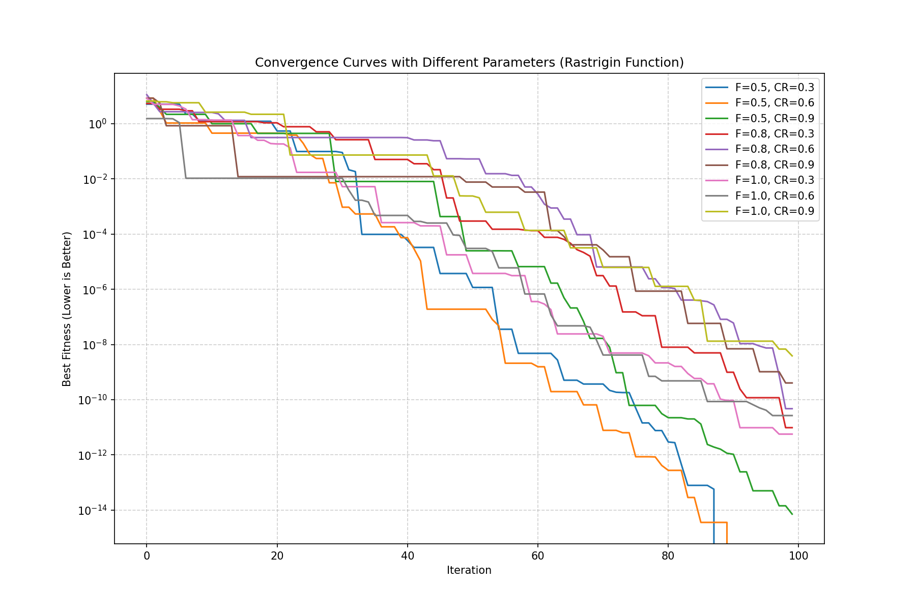
推荐组合:F=0.5, CR=0.6
-
关于 F (缩放因子/变异强度):
-
F=0.5 (较小):步长较小,精细搜索能力强,收敛速度通常较快,但在极度复杂的多峰函数中容易陷入局部最优。
-
F=1.0 (较大):步长很大,扰动剧烈。虽然全局探索能力强,不容易陷入局部最优,但收敛非常慢,且很难精确收敛到绝对极值点(在最优解附近震荡)。
-
-
关于 CR (交叉概率):
-
CR=0.9 (较大):意味着子代大部分基因来自变异向量(即更多地采纳了种群差异信息)。这通常能显著加快收敛速度。
-
CR=0.3 (较小):意味着子代大部分保留父代基因。算法变得非常保守,收敛速度会变慢。
-
总结:
-
最快收敛/最稳定:通常出现在F=0.5, CR=0.6。这个组合利用高交叉率快速传递优良基因,同时较小的F 保证了后期的精细挖掘。
-
最慢/最不稳定:通常是F=1.0, CR=0.3。大步长导致乱跳,低交叉导致进化缓慢。