

实践一
任务1:实现非支配排序
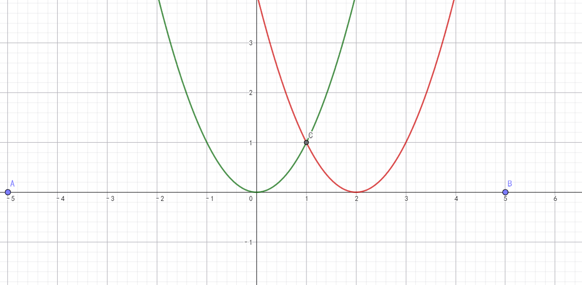
输入一组二维点→分 Rank 1、Rank 2.
任务2:计算拥挤距离
观察高/低距离点的差异
任务3:实现迷你 NSGA-II
种群 30、选代20代→输出不断逼近的前沿图
代码
import numpy as np
import matplotlib.pyplot as plt
import random
# ==========================================
# 0. 基础定义与测试问题 (Minimization Problem)
# ==========================================
# 目标函数定义
# 变量 x 范围 [-5, 5]
# 目标 f1 = x^2
# 目标 f2 = (x - 2)^2
def evaluate_objectives(x):
f1 = x**2
f2 = (x - 2)**2
return [f1, f2]
class Individual:
def __init__(self, x=None):
# 基因 (变量)
if x is None:
self.x = random.uniform(-5, 5)
else:
self.x = x
# 目标函数值 (二维点)
self.objs = evaluate_objectives(self.x)
# NSGA-II 属性
self.rank = 0
self.distance = 0.0
self.domination_count = 0
self.dominated_solutions = []
def __repr__(self):
return f"Ind(x={self.x:.2f}, objs={self.objs}, rank={self.rank}, dist={self.distance:.2f})"
# ==========================================
# 1. 核心算法组件
# ==========================================
# --- 任务 1: 实现非支配排序 ---
def fast_non_dominated_sort(population):
fronts = [[]]
for p in population:
p.dominated_solutions = []
p.domination_count = 0
for q in population:
# 判断 p 是否支配 q (Minimization)
# p 支配 q 的条件:
# 1. p 在所有目标上 <= q
# 2. p 至少在一个目标上 < q
p_dominates_q = (p.objs[0] <= q.objs[0] and p.objs[1] <= q.objs[1]) and \
(p.objs[0] < q.objs[0] or p.objs[1] < q.objs[1])
q_dominates_p = (q.objs[0] <= p.objs[0] and q.objs[1] <= p.objs[1]) and \
(q.objs[0] < p.objs[0] or q.objs[1] < p.objs[1])
if p_dominates_q:
p.dominated_solutions.append(q)
elif q_dominates_p:
p.domination_count += 1
if p.domination_count == 0:
p.rank = 1
fronts[0].append(p)
i = 0
while len(fronts[i]) > 0:
next_front = []
for p in fronts[i]:
for q in p.dominated_solutions:
q.domination_count -= 1
if q.domination_count == 0:
q.rank = i + 2
next_front.append(q)
i += 1
fronts.append(next_front)
return fronts[:-1] # 移除最后一个空层
# --- 任务 2: 计算拥挤距离 ---
def calculate_crowding_distance(front):
l = len(front)
if l == 0: return
# 初始化距离为0
for p in front:
p.distance = 0
# 对每个目标进行计算
num_objs = len(front[0].objs)
for m in range(num_objs):
# 根据第 m 个目标值排序
front.sort(key=lambda x: x.objs[m])
# 边界点距离设为无穷大 (Inf)
front[0].distance = float('inf')
front[l-1].distance = float('inf')
# 获取最大最小值用于归一化
m_min = front[0].objs[m]
m_max = front[l-1].objs[m]
if m_max == m_min: continue
# 计算中间点的距离
for i in range(1, l-1):
front[i].distance += (front[i+1].objs[m] - front[i-1].objs[m]) / (m_max - m_min)
# ==========================================
# 2. 辅助函数 (选择与交叉变异)
# ==========================================
def tournament_selection(pop):
# 锦标赛选择:随机选2个,留最好的
a, b = random.sample(pop, 2)
# 优先选 Rank 小的 (非支配等级高)
if a.rank < b.rank: return a
elif b.rank < a.rank: return b
else:
# Rank 一样选 Distance 大的 (拥挤度低,更稀疏)
if a.distance > b.distance: return a
else: return b
def create_offspring(parent1, parent2):
# 模拟二进制交叉 (SBX) 的简化版 -> 线性组合
alpha = random.random()
child_x = alpha * parent1.x + (1 - alpha) * parent2.x
# 变异 (高斯变异)
if random.random() < 0.1:
child_x += random.gauss(0, 0.5)
child_x = max(-5, min(5, child_x)) # 边界截断
return Individual(child_x)
# ==========================================
# 3. 功能展示函数 (对应你的具体要求)
# ==========================================
def demo_tasks():
print("\n" + "="*50)
print(" 🎯 第一部分:手动验证核心算法逻辑")
print("="*50)
# 构造特定的测试点方便观察
# P1(x=1): [1, 1] -> 均衡型
# P2(x=0): [0, 4] -> 偏科型 (边界)
# P3(x=2): [4, 0] -> 偏科型 (边界)
# P4(x=3): [9, 1] -> 被 P1 支配
# P5(x=4): [16,4] -> 被所有人支配
demo_pop = [Individual(1), Individual(0), Individual(2), Individual(3), Individual(4)]
# --- 演示任务 1 ---
print(f"\n📝 任务 1: 实现非支配排序")
print(f"👉 输入一组二维点 → 分 Rank 1、Rank 2...")
print("-" * 40)
print("【输入数据】:")
for i, p in enumerate(demo_pop):
print(f" 点 {i} (x={p.x}): {p.objs}")
fronts = fast_non_dominated_sort(demo_pop)
print("\n【输出分层结果】:")
for i, front in enumerate(fronts):
front_objs = [p.objs for p in front]
print(f" 🏆 Rank {i + 1}: {front_objs}")
# --- 演示任务 2 ---
print(f"\n📝 任务 2: 计算拥挤距离")
print(f"👉 观察高/低距离点的差异")
print("-" * 40)
# 只看 Rank 1 层
rank1_front = fronts[0]
calculate_crowding_distance(rank1_front)
rank1_front.sort(key=lambda p: p.objs[0]) # 按目标1排序方便看
print("【Rank 1 层的计算结果】:")
print(f" {'坐标 (f1, f2)':<18} | {'拥挤距离':<10} | {'差异说明'}")
print("-" * 60)
for p in rank1_front:
if p.distance == float('inf'):
note = "🔥 高距离 (边界点,必须保留)"
dist_str = "Inf"
else:
note = "💧 低距离 (中间点,会被优先比较)"
dist_str = f"{p.distance:.4f}"
print(f" {str(p.objs):<18} | {dist_str:<10} | {note}")
print("\n")
# ==========================================
# 4. 任务 3: Mini NSGA-II 主程序
# ==========================================
def mini_nsga_ii():
print("="*50)
print(" 🚀 第二部分:任务 3 - 实现迷你 NSGA-II")
print("="*50)
# 参数设置
POP_SIZE = 30
GENERATIONS = 20
# 初始化
population = [Individual() for _ in range(POP_SIZE)]
history = []
print(f"开始进化: 种群 {POP_SIZE}, 迭代 {GENERATIONS} 代")
for gen in range(GENERATIONS):
# 排序与距离计算
fronts = fast_non_dominated_sort(population)
for front in fronts:
calculate_crowding_distance(front)
# 记录首末代数据
if gen == 0 or gen == GENERATIONS - 1:
history.append([p.objs for p in population])
# 生成子代
offspring = []
while len(offspring) < POP_SIZE:
p1 = tournament_selection(population)
p2 = tournament_selection(population)
child = create_offspring(p1, p2)
offspring.append(child)
# 精英保留 (核心逻辑)
combined_pop = population + offspring
fronts = fast_non_dominated_sort(combined_pop)
new_pop = []
for front in fronts:
calculate_crowding_distance(front)
if len(new_pop) + len(front) <= POP_SIZE:
new_pop.extend(front)
else:
# 按照拥挤距离从大到小排序,填满剩余位置
front.sort(key=lambda x: x.distance, reverse=True)
needed = POP_SIZE - len(new_pop)
new_pop.extend(front[:needed])
break
population = new_pop
# 打印每一代的最佳层级数量
rank1_count = len([p for p in population if p.rank == 1])
print(f" Gen {gen+1}: Rank 1 个体数 = {rank1_count}")
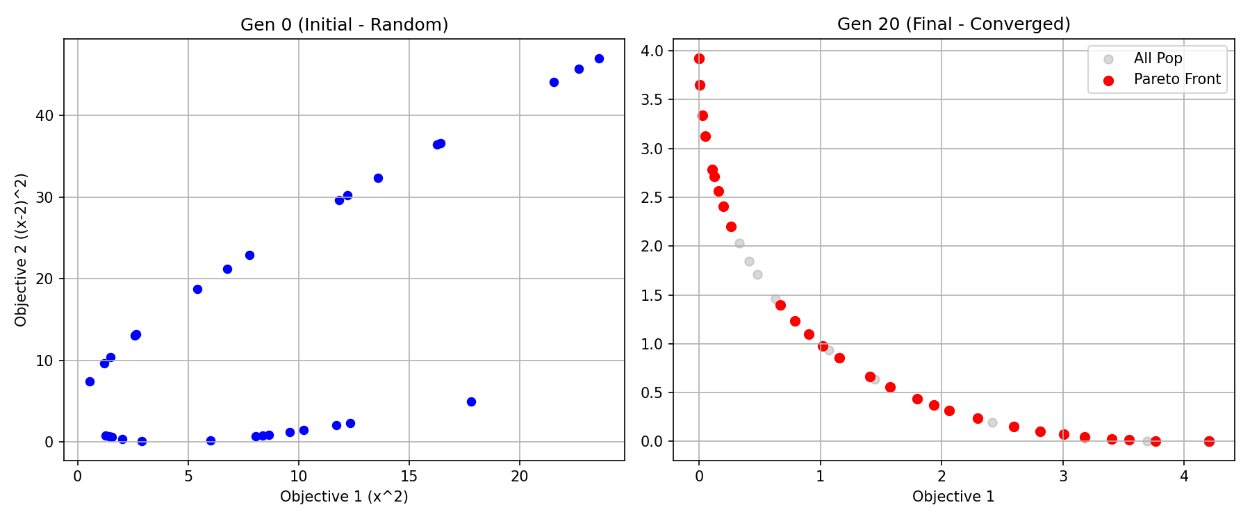
# --- 绘图 ---
print("\n正在绘图展示不断逼近的前沿图...")
plt.figure(figsize=(12, 5))
# 图1: 初始种群
init_objs = np.array(history[0])
plt.subplot(1, 2, 1)
plt.scatter(init_objs[:,0], init_objs[:,1], c='blue', s=30, label='Solutions')
plt.title('Gen 0 (Initial - Random)')
plt.xlabel('Objective 1 (x^2)')
plt.ylabel('Objective 2 ((x-2)^2)')
plt.grid(True)
# 图2: 最终种群
final_objs = np.array(history[-1])
rank1_objs = np.array([p.objs for p in population if p.rank == 1])
plt.subplot(1, 2, 2)
plt.scatter(final_objs[:,0], final_objs[:,1], c='gray', alpha=0.3, label='All Pop')
plt.scatter(rank1_objs[:,0], rank1_objs[:,1], c='red', s=40, label='Pareto Front')
plt.title(f'Gen {GENERATIONS} (Final - Converged)')
plt.xlabel('Objective 1')
plt.grid(True)
plt.legend()
plt.tight_layout()
plt.show()
# ==========================================
# 程序入口
# ==========================================
if __name__ == "__main__":
# 1. 先运行文本演示 (满足你对任务1、2的输出要求)
demo_tasks()
# 2. 再运行完整算法 (满足任务3的输出要求)
mini_nsga_ii()输出
==================================================
 🎯 第一部分:手动验证核心算法逻辑
==================================================

📝 任务 1: 实现非支配排序
👉 输入一组二维点 → 分 Rank 1、Rank 2...
----------------------------------------
【输入数据】:
  点 0 (x=1): [1, 1]
  点 1 (x=0): [0, 4]
  点 2 (x=2): [4, 0]
  点 3 (x=3): [9, 1]
  点 4 (x=4): [16, 4]

【输出分层结果】:
  🏆 Rank 1: [[1, 1], [0, 4], [4, 0]]
  🏆 Rank 2: [[9, 1]]
  🏆 Rank 3: [[16, 4]]

📝 任务 2: 计算拥挤距离
👉 观察高/低距离点的差异
----------------------------------------
【Rank 1 层的计算结果】:
  坐标 (f1, f2)        | 拥挤距离       | 差异说明
------------------------------------------------------------
  [0, 4]             | Inf        | 🔥 高距离 (边界点,必须保留)
  [1, 1]             | 2.0000     | 💧 低距离 (中间点,会被优先比较)
  [4, 0]             | Inf        | 🔥 高距离 (边界点,必须保留)


==================================================
 🚀 第二部分:任务 3 - 实现迷你 NSGA-II
==================================================
开始进化: 种群 30, 迭代 20 代
  Gen 1: Rank 1 个体数 = 17
  Gen 2: Rank 1 个体数 = 30
  Gen 3: Rank 1 个体数 = 30
  Gen 4: Rank 1 个体数 = 30
  Gen 5: Rank 1 个体数 = 30
  Gen 6: Rank 1 个体数 = 30
  Gen 7: Rank 1 个体数 = 30
  Gen 8: Rank 1 个体数 = 30
  Gen 9: Rank 1 个体数 = 30
  Gen 10: Rank 1 个体数 = 30
  Gen 11: Rank 1 个体数 = 30
  Gen 12: Rank 1 个体数 = 30
  Gen 13: Rank 1 个体数 = 30
  Gen 14: Rank 1 个体数 = 30
  Gen 15: Rank 1 个体数 = 30
  Gen 16: Rank 1 个体数 = 30
  Gen 17: Rank 1 个体数 = 30
  Gen 18: Rank 1 个体数 = 30
  Gen 19: Rank 1 个体数 = 30
  Gen 20: Rank 1 个体数 = 30

正在绘图展示不断逼近的前沿图...
可视化
实践二
-
随机生成 50 个二维解 x \in [0,4]
-
计算其 f_1 \space f_2
-
通过支配关系筛选出帕累托最优解
-
绘制解集与帕累托前沿
输出
-
帕累托点图
-
不同 Pareto 解的意义
代码
import numpy as np
import matplotlib.pyplot as plt
import random

# ========= 中文正常显示 =========
plt.rcParams['font.sans-serif'] = ['SimHei']   # 正常显示中文
plt.rcParams['axes.unicode_minus'] = False     # 正常显示负号

# ============================
# 步骤 1 & 2: 定义问题与生成数据
# ============================
def evaluate_objectives(x):
    # f1 = x^2
    # f2 = (x-2)^2
    return [x**2, (x-2)**2]

class Solution:
    def __init__(self, x_val):
        self.x = x_val
        self.objs = evaluate_objectives(self.x)
        self.is_pareto = False # 标记是否为帕累托最优

# 1. 随机生成 50 个解,范围 [0, 4]
N = 50
solutions = []
print(f"正在生成 {N} 个随机解 (x ∈ [0, 4])...")
for _ in range(N):
    x_rand = random.uniform(0, 4)
    solutions.append(Solution(x_rand))

# ============================
# 步骤 3: 筛选帕累托最优解
# ============================
# 暴力筛选法
for i in range(N):
    p = solutions[i]
    dominated = False
    for j in range(N):
        if i == j: continue
        q = solutions[j]
        # 如果 q 支配 p (q 的两项指标都 <= p,且至少有一项更小)
        if (q.objs[0] <= p.objs[0] and q.objs[1] <= p.objs[1]) and \
           (q.objs[0] < p.objs[0] or q.objs[1] < p.objs[1]):
            dominated = True
            break

    if not dominated:
        p.is_pareto = True

# 提取帕累托解
pareto_solutions = [s for s in solutions if s.is_pareto]

# ============================
# 【新增】: 输出最优解列表
# ============================
# 为了看清楚,我们按变量 x 从小到大排序
pareto_solutions.sort(key=lambda s: s.x)

print("\n" + "="*60)
print(f"筛选完成!共找到 {len(pareto_solutions)} 个帕累托最优解 (Pareto Optimal):")
print("="*60)
print(f"{'变量 x':<15} | {'f1 (x^2)':<15} | {'f2 ((x-2)^2)':<15}")
print("-" * 60)

for s in pareto_solutions:
    # 格式化输出,保留4位小数
    print(f"{s.x:<15.4f} | {s.objs[0]:<15.4f} | {s.objs[1]:<15.4f}")

print("="*60 + "\n")

# ============================
# 步骤 4: 绘制解集与帕累托前沿
# ============================
plt.figure(figsize=(9, 6))

# 提取坐标
all_f1 = [s.objs[0] for s in solutions]
all_f2 = [s.objs[1] for s in solutions]
pareto_f1 = [s.objs[0] for s in pareto_solutions]
pareto_f2 = [s.objs[1] for s in pareto_solutions]

# 绘制所有解 (灰色)
plt.scatter(all_f1, all_f2, color='gray', alpha=0.5, s=40, label='普通解 (Dominated)')

# 绘制帕累托解 (红色)
plt.scatter(pareto_f1, pareto_f2, color='red', s=80, zorder=5, label='帕累托最优解 (Pareto Set)')
plt.plot(pareto_f1, pareto_f2, color='red', linestyle='--', alpha=0.5) # 连线

plt.title(f'Pareto Front Visualization (N={N})')
plt.xlabel('Objective f1 ($x^2$)')
plt.ylabel('Objective f2 ($(x-2)^2$)')
plt.legend()
plt.grid(True)
plt.tight_layout()
plt.show()
输出
正在生成 50 个随机解 (x ∈ [0, 4])...

============================================================
筛选完成!共找到 30 个帕累托最优解 (Pareto Optimal):
============================================================
变量 x            | f1 (x^2)        | f2 ((x-2)^2)
------------------------------------------------------------
0.2120          | 0.0449          | 3.1969
0.2623          | 0.0688          | 3.0195
0.2660          | 0.0707          | 3.0069
0.2690          | 0.0724          | 2.9963
0.3068          | 0.0941          | 2.8669
0.3241          | 0.1050          | 2.8087
0.3361          | 0.1130          | 2.7686
0.4134          | 0.1709          | 2.5174
0.5375          | 0.2889          | 2.1388
0.6593          | 0.4346          | 1.7976
0.7734          | 0.5981          | 1.5047
0.9856          | 0.9715          | 1.0289
1.0504          | 1.1034          | 0.9017
1.2918          | 1.6687          | 0.5016
1.3478          | 1.8165          | 0.4254
1.3813          | 1.9080          | 0.3828
1.4069          | 1.9792          | 0.3518
1.4264          | 2.0346          | 0.3290
1.4482          | 2.0974          | 0.3044
1.4521          | 2.1086          | 0.3002
1.5455          | 2.3884          | 0.2066
1.5621          | 2.4401          | 0.1918
1.6341          | 2.6702          | 0.1339
1.6544          | 2.7371          | 0.1194
1.6706          | 2.7910          | 0.1085
1.6889          | 2.8525          | 0.0968
1.7037          | 2.9026          | 0.0878
1.7261          | 2.9795          | 0.0750
1.8834          | 3.5472          | 0.0136
2.0572          | 4.2321          | 0.0033
============================================================
可视化
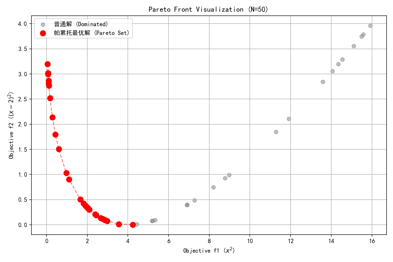
帕累托最优解集(Pareto Optimal Set)代表了在多目标冲突下的最佳权衡(Trade-offs)状态。
前沿上的每一个点都是不可被优化的:这意味着你不可能在不牺牲目标 A 的情况下提升目标 B。
-
前沿两端的解代表了极端偏好(例如:只在这个位置f_1 最小,但f_2 极大)。
-
前沿中间的解代表了均衡折中。
帕累托解集的意义在于为决策者提供了一组“最有效率的候选方案”,决策者可以根据实际需求(如更看重成本还是性能)从中选取最合适的一个,而非盲目寻找不存在的完美解。